Tool for placing virtual stations in demand-responsive transport systems in villages by defining and minimizing a global energy (drtplanr, name is inspired by stplanr). The station locations are randomly initialized in the street network and iteratively optimized based on the reachable population in combination with walking and driving times.
The model in the package example optimizes the positions of virtual stations in an assumed on-demand shuttle service for the community of Jegenstorf in Bern, Switzerland.
Example data sets
Load the package example data sets:
- aoi: Area of Interest - 3 min driving time isochrone around the station of Jegenstorf, Bern.
- pop: Centroids of population and structural business hectare grid statistis (BfS).
aoi <-
  sf::st_read(system.file("example.gpkg", package="drtplanr"), layer = "aoi")
#> Reading layer `aoi' from data source `/home/runner/work/_temp/Library/drtplanr/example.gpkg' using driver `GPKG'
#> Simple feature collection with 1 feature and 6 fields
#> geometry type:  POLYGON
#> dimension:      XY
#> bbox:           xmin: 7.4947 ymin: 47.0366 xmax: 7.5359 ymax: 47.0599
#> geographic CRS: WGS 84

pop <-
  sf::st_read(system.file("example.gpkg", package="drtplanr"), layer = "pop")
#> Reading layer `pop' from data source `/home/runner/work/_temp/Library/drtplanr/example.gpkg' using driver `GPKG'
#> Simple feature collection with 150 features and 4 fields
#> geometry type:  POINT
#> dimension:      XY
#> bbox:           xmin: 7.496534 ymin: 47.04012 xmax: 7.524167 ymax: 47.0581
#> geographic CRS: WGS 84

m <-
  mapview(aoi, alpha.region = 0, layer.name = "AOI", homebutton = FALSE) +
  mapview(pop, zcol = "n", alpha = 0, layer.name = "Population", homebutton = FALSE)
m
Initialize drtm model
Create a new demand reponsive transport model for the aoi ‘Jegenstorf’, with 10 randomly initialized virtual on-demand stations.
m <- drt_drtm(
  model_name = "Jegenstorf",
  aoi = aoi, pop = pop,
  n_vir = 15, m_seg = 100
)
#> 2020-05-25 18:30:15 Get data from OSM: Streets 'roa', bus stops and rail stations 'sta'
#> Request failed [429]. Retrying in 1.6 seconds...
#> Request failed [429]. Retrying in 1.6 seconds...
#> 2020-05-25 18:31:25 Create routing graphs for 'foot' and 'mcar'
#> 2020-05-25 18:31:25 Mask layers 'roa', 'pop' and 'sta' by 'aoi'
#> 2020-05-25 18:31:25 Extract possible station locations 'seg' from street segments
#> 2020-05-25 18:31:25 Route driving times of 'seg' to the rail stations
#> 2020-05-25 18:31:27 Map stations 'sta' to segments 'seg' and set as constant
m
#> ================================================================================
#> Demand-responsive transport model 'Jegenstorf'
#>
#> ______________________________________ i __________________ dE/di ______________
#> Iteration:                                                0                  NaN
#> ______________________________________ initial ____________ current ____________
#> Energy:                                            208127.4             208127.4
#> ______________________________________ existing ___________ virtual ____________
#> Stations:                                                10                   15
#> ______________________________________ lng ________________ lat ________________
#> BBox:                             min:              7.49470             47.03660
#>                                   max:              7.53590             47.05990
Minimze the energy of the model
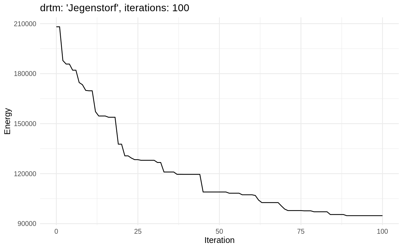
Iterate the model 100 times, where every iteration consists of:
- Relocate a virtual station randomly on the road segments.
- Calculate the new global energy of the model using the routing graphs.
- If the energy is lower than previuos iteration: Keep the new location of the virtual station; otherwise: Reset to the previous location.
m1 <- drt_iterate(m, 100)
Print model summary:
m1
#> ================================================================================
#> Demand-responsive transport model 'Jegenstorf'
#>
#> ______________________________________ i __________________ dE/di ______________
#> Iteration:                                              100                  NaN
#> ______________________________________ initial ____________ current ____________
#> Energy:                                            208127.4              94790.2
#> ______________________________________ existing ___________ virtual ____________
#> Stations:                                                10                   15
#> ______________________________________ lng ________________ lat ________________
#> BBox:                             min:              7.49470             47.03660
#>                                   max:              7.53590             47.05990
Plotting
Station map
drt_map(m1)
#> 2020-05-25 18:31:35 Print station map
Iterate again
The model state is saved in the model. This allows making copies and store different stages of the optimization.
m2 <- drt_iterate(m1, 900)
Print model summary:
m2
#> ================================================================================
#> Demand-responsive transport model 'Jegenstorf'
#>
#> ______________________________________ i __________________ dE/di ______________
#> Iteration:                                             1000                  NaN
#> ______________________________________ initial ____________ current ____________
#> Energy:                                            165303.3              51821.1
#> ______________________________________ existing ___________ virtual ____________
#> Stations:                                                10                   15
#> ______________________________________ lng ________________ lat ________________
#> BBox:                             min:              7.49470             47.03660
#>                                   max:              7.53590             47.05990
Visualize results
drt_plot(m2)
#> 2020-05-25 18:31:36 Print energy plot

drt_map(m2)
#> 2020-05-25 18:31:36 Print station map
Export and import
The drtplanr has functions to import and export the drtm objects. Furthermore graphics of the energy plot and the station map can be exported as images (.png).
# Export model
drt_export(m2, path = getwd())

# Import model
m2 <- drt_import("Jegenstorf_i1000.RData")

# Save graphics
drt_save_graphics(m2, path = getwd())